In this lecture we discuss under which assumptions the OLS (Ordinary Least Squares) estimator has desirable statistical properties such as consistency and asymptotic normality.
Table of contents
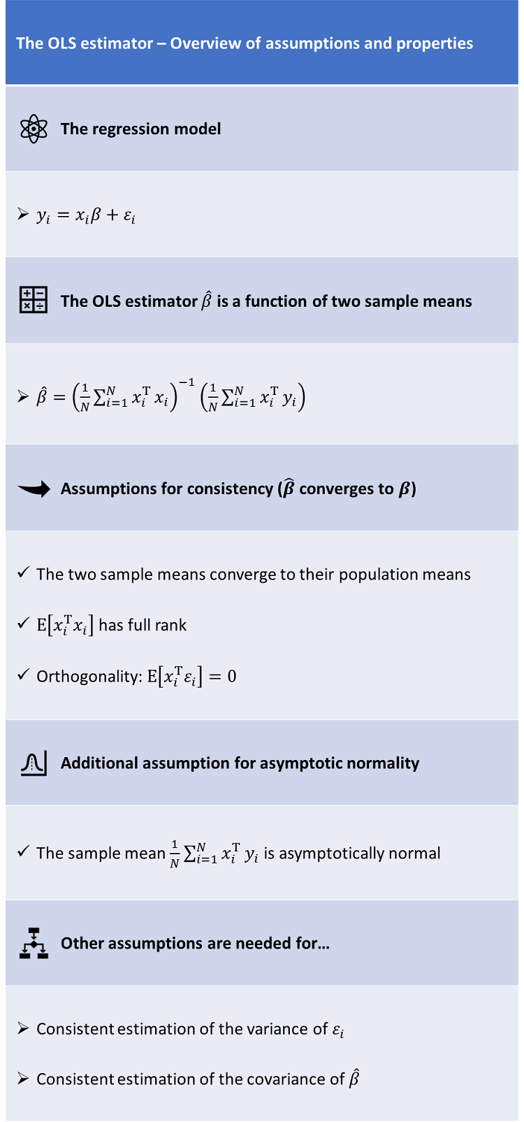
Consider the linear regression model where:
We assume to observe a sample of realizations, so that the vector of all outputs
is an vector, the design matrix is an matrix, and the vector of error terms is an vector.
The OLS estimator is the vector of regression coefficients that minimizes the sum of squared residuals:
As proved in the lecture on Linear regression, if the design matrix has full rank, then the OLS estimator is computed as follows:
The OLS estimator can be written as where is the sample mean of the matrix and is the sample mean of the matrix .
In this section we are going to propose a set of conditions that are sufficient for the consistency of the OLS estimator, that is, for the convergence in probability of to the true value .
The first assumption we make is that the sample means in the OLS formula converge to their population counterparts, which is formalized as follows.
Assumption 1 (convergence): both the sequence and the sequence satisfy sets of conditions that are sufficient for the convergence in probability of their sample means to the population means and , which do not depend on .
For example, the sequences and could be assumed to satisfy the conditions of Chebyshev's Weak Law of Large Numbers for correlated sequences, which are quite mild (basically, it is only required that the sequences are covariance stationary and that their auto-covariances are zero on average).
The second assumption we make is a rank assumption (sometimes also called identification assumption).
Assumption 2 (rank): the square matrix has full rank (as a consequence, it is invertible).
The third assumption we make is that the regressors are orthogonal to the error terms .
Assumption 3 (orthogonality): For each , and are orthogonal, that is,
It is then straightforward to prove the following proposition.
Proposition If Assumptions 1, 2 and 3 are satisfied, then the OLS estimator is a consistent estimator of .
![[eq20]](https://www.statlect.com/images/OLS-estimator-properties__47.png)
Let us make explicit the dependence of the estimator on the sample size and denote by the OLS estimator obtained when the sample size is equal to By Assumption 1 and by the Continuous Mapping theorem, we have that the probability limit of is Now, if we pre-multiply the regression equation by and we take expected values, we get But by Assumption 3, it becomes or which implies that
We now introduce a new assumption, and we use it to prove the asymptotic normality of the OLS estimator.
The assumption is as follows.
Assumption 4 (Central Limit Theorem): the sequence satisfies a set of conditions that are sufficient to guarantee that a Central Limit Theorem applies to its sample mean
For a review of some of the conditions that can be imposed on a sequence to guarantee that a Central Limit Theorem applies to its sample mean, you can go to the lecture on the Central Limit Theorem.
In any case, remember that if a Central Limit Theorem applies to , then, as tends to infinity, converges in distribution to a multivariate normal distribution with mean equal to and covariance matrix equal to
With Assumption 4 in place, we are now able to prove the asymptotic normality of the OLS estimator.
Proposition If Assumptions 1, 2, 3 and 4 are satisfied, then the OLS estimator is asymptotically multivariate normal with mean equal to and asymptotic covariance matrix equal to that is, where has been defined above.
As in the proof of consistency, the dependence of the estimator on the sample size is made explicit, so that the OLS estimator is denoted by . First of all, we have ![[eq34]](https://www.statlect.com/images/OLS-estimator-properties__67.png) where, in the last step, we have used the fact that, by Assumption 3, . Note that, by Assumption 1 and the Continuous Mapping theorem, we have Furthermore, by Assumption 4, we have that converges in distribution to a multivariate normal random vector having mean equal to and covariance matrix equal to . Thus, by Slutski's theorem, we have that
where, in the last step, we have used the fact that, by Assumption 3, . Note that, by Assumption 1 and the Continuous Mapping theorem, we have Furthermore, by Assumption 4, we have that converges in distribution to a multivariate normal random vector having mean equal to and covariance matrix equal to . Thus, by Slutski's theorem, we have that ![[eq38]](https://www.statlect.com/images/OLS-estimator-properties__73.png) converges in distribution to a multivariate normal vector with mean equal to and covariance matrix equal to
converges in distribution to a multivariate normal vector with mean equal to and covariance matrix equal to
We now discuss the consistent estimation of the variance of the error terms.
Here is an additional assumption.
Assumption 5: the sequence satisfies a set of conditions that are sufficient for the convergence in probability of its sample mean to the population mean which does not depend on .
If this assumption is satisfied, then the variance of the error terms can be estimated by the sample variance of the residuals where
Proposition Under Assumptions 1, 2, 3, and 5, it can be proved that is a consistent estimator of .
![[eq49]](https://www.statlect.com/images/OLS-estimator-properties__89.png)
Let us make explicit the dependence of the estimators on the sample size and denote by and the estimators obtained when the sample size is equal to By Assumption 1 and by the Continuous Mapping theorem, we have that the probability limit of is where: in steps and we have used the Continuous Mapping Theorem; in step we have used Assumption 5; in step we have used the fact that because is a consistent estimator of , as proved above.
We have proved that the asymptotic covariance matrix of the OLS estimator is where the long-run covariance matrix is defined by
Usually, the matrix needs to be estimated because it depends on quantities ( and ) that are not known.
The next proposition characterizes consistent estimators of .
Proposition If Assumptions 1, 2, 3, 4 and 5 are satisfied, and a consistent estimator of the long-run covariance matrix is available, then the asymptotic variance of the OLS estimator is consistently estimated by
This is proved as follows where: in step we have used the Continuous Mapping theorem; in step we have used the hypothesis that is a consistent estimator of the long-run covariance matrix and the fact that, by Assumption 1, the sample mean of the matrix is a consistent estimator of , that is
Thus, in order to derive a consistent estimator of the covariance matrix of the OLS estimator, we need to find a consistent estimator of the long-run covariance matrix . How to do this is discussed in the next section.
The estimation of requires some assumptions on the covariances between the terms of the sequence .
In order to find a simpler expression for , we make the following assumption.
Assumption 6: the sequence is serially uncorrelated, that is, and weakly stationary, that is, does not depend on .
Remember that in Assumption 3 (orthogonality) we also ask that
We now derive simpler expressions for .
Proposition Under Assumptions 3 (orthogonality), the long-run covariance matrix satisfies
![[eq67]](https://www.statlect.com/images/OLS-estimator-properties__128.png)
This is proved as follows:
Proposition Under Assumptions 3 (orthogonality) and 6 (no serial correlation), the long-run covariance matrix satisfies
![[eq69]](https://www.statlect.com/images/OLS-estimator-properties__131.png)
The proof is as follows:
Thanks to assumption 6, we can also derive an estimator of .
Proposition Suppose that Assumptions 1, 2, 3, 4 and 6 are satisfied, and that is consistently estimated by the sample mean Then, the long-run covariance matrix is consistently estimated by
![[eq73]](https://www.statlect.com/images/OLS-estimator-properties__137.png)
We have where in the last step we have applied the Continuous Mapping theorem separately to each entry of the matrices in square brackets, together with the fact that To see how this is done, consider, for example, the matrix Then, the entry at the intersection of its -th row and -th column is and
When the assumptions of the previous proposition hold, the asymptotic covariance matrix of the OLS estimator is
As a consequence, the covariance of the OLS estimator can be approximated by which is known as heteroskedasticity-robust estimator.
A further assumption is often made, which allows us to further simplify the expression for the long-run covariance matrix.
Assumption 7: the error terms are conditionally homoskedastic:
This assumption has the following implication.
Proposition Suppose that Assumptions 1, 2, 3, 4, 5, 6 and 7 are satisfied. Then, the long-run covariance matrix is consistently estimated by
![[eq82]](https://www.statlect.com/images/OLS-estimator-properties__149.png)
First of all, we have that But we know that, by Assumption 1, is consistently estimated by and by Assumptions 1, 2, 3 and 5, is consistently estimated by Therefore, by the Continuous Mapping theorem, the long-run covariance matrix is consistently estimated by
When the assumptions of the previous proposition hold, the asymptotic covariance matrix of the OLS estimator is
As a consequence, the covariance of the OLS estimator can be approximated by which is the same estimator derived in the normal linear regression model.
The assumptions above can be made even weaker (for example, by relaxing the hypothesis that is uncorrelated with ), at the cost of facing more difficulties in estimating the long-run covariance matrix.
For a review of the methods that can be used to estimate , see, for example, Den and Levin (1996).
The lecture entitled Linear regression - Hypothesis testing discusses how to carry out hypothesis tests on the coefficients of a linear regression model in the cases discussed above, that is, when the OLS estimator is asymptotically normal and a consistent estimator of the asymptotic covariance matrix is available.
Haan, Wouter J. Den, and Andrew T. Levin (1996). "Inferences from parametric and non-parametric covariance matrix estimation procedures." Technical Working Paper Series, NBER.
Taboga, Marco (2021). "Properties of the OLS estimator", Lectures on probability theory and mathematical statistics. Kindle Direct Publishing. Online appendix. https://www.statlect.com/fundamentals-of-statistics/OLS-estimator-properties.
Most of the learning materials found on this website are now available in a traditional textbook format.
Featured pages